年度
- 100
- 100
- 100
- 100
- 100
- 100
- 100
- 100
- 100
- 100
- 100
- 100
- 100
- 100
- 100
- 100
- 100
- 99
- 99
- 99
- 99
- 99
- 99
- 99
- 99
- 99
- 99
- 99
- 99
- 99
- 99
- 99
- 99
- 99
- 99
- 99
- 99
- 99
- 99
- 99
- 99
- 98
- 98
- 98
- 98
- 98
- 98
- 98
- 98
- 98
- 98
- 98
- 98
- 98
- 98
- 98
- 98
- 98
- 98
- 98
- 98
- 98
- 98
- 98
- 98
- 98
- 98
- 98
- 98
- 98
- 98
- 98
- 98
- 97
- 97
- 97
- 97
- 97
- 97
- 97
- 97
- 97
- 97
- 97
- 97
- 97
- 97
- 97
- 97
- 97
- 97
- 97
- 97
- 97
- 97
- 97
- 97
- 97
- 97
- 97
- 97
- 96
- 96
- 96
- 96
- 96
- 96
- 96
- 96
- 96
- 96
- 96
- 96
- 96
- 96
- 96
- 96
- 96
- 96
- 96
- 96
- 96
- 96
- 96
- 96
- 96
- 96
- 96
- 96
- 96
- 96
- 96

- 1.
- 題型:問答題
- 難易度:尚未記錄
- 2.
- 題型:問答題
- 難易度:尚未記錄
- 3.
- 題型:問答題
- 難易度:尚未記錄
- 4.
- 題型:問答題
- 難易度:尚未記錄
- 5.
- 題型:問答題
- 難易度:尚未記錄
- 6.
- 題型:問答題
- 難易度:尚未記錄
- 7.
- 題型:問答題
- 難易度:尚未記錄
- 8.
- 題型:問答題
- 難易度:尚未記錄
- 9.
- 題型:問答題
- 難易度:尚未記錄
- 10.
- 題型:問答題
- 難易度:尚未記錄
- 11.
- 題型:問答題
- 難易度:尚未記錄
- 12.
Let {−0.8, −0.4, −0.2, 0.6} be a sample from a uniform distribution on [−1, 1]. Based on
this sample, please generate (simulate) a sample which is from an exponential
distribution 0.5e−x / 2 .(10%)
- 題型:問答題
- 難易度:尚未記錄
- 13.
- 題型:問答題
- 難易度:尚未記錄
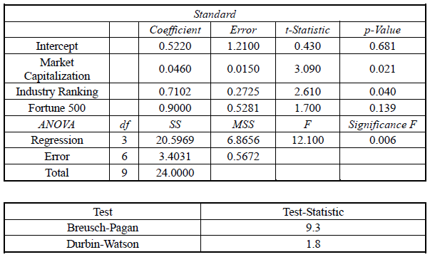
Multiple regression was used to explain stock returns using the following variables:
Dependent variable:
RET = annual stock returns (%)
Independent variables:
MKT = Market capitalization = Market capitalization / $1.0 million
IND = Industry quartile ranking (IND = 4 is the highest ranking)
FORT = Fortune 500 firm, where {FORT = 1 if the stock is that of a Fortune 500
firm, FORT = 0 if not a Fortune 500 stock}
The regression results are presented in the tables below
- 14.
The expected amount of the stock return attributable to it being a Fortune 500 stock
is closest to:- (A)
0.522.
- (B)
0.046
- (C)
0.710
- (D)
0.900
- 題型:單選題
- 難易度:尚未記錄
- 登入看解答
Multiple regression was used to explain stock returns using the following variables:
Dependent variable:
RET = annual stock returns (%)
Independent variables:
MKT = Market capitalization = Market capitalization / $1.0 million
IND = Industry quartile ranking (IND = 4 is the highest ranking)
FORT = Fortune 500 firm, where {FORT = 1 if the stock is that of a Fortune 500
firm, FORT = 0 if not a Fortune 500 stock}
The regression results are presented in the tables below
- 15.
The expected return on the stock of a firm that is not in the Fortune 500, has a
market capitalization of $5 million, and is in an industry with a rank of 3 is closest to:- (A)
2.88%.
- (B)
3.98%.
- (C)
1.42%.
- (D)
2.10%
- 題型:單選題
- 難易度:尚未記錄
- 登入看解答
Multiple regression was used to explain stock returns using the following variables:
Dependent variable:
RET = annual stock returns (%)
Independent variables:
MKT = Market capitalization = Market capitalization / $1.0 million
IND = Industry quartile ranking (IND = 4 is the highest ranking)
FORT = Fortune 500 firm, where {FORT = 1 if the stock is that of a Fortune 500
firm, FORT = 0 if not a Fortune 500 stock}
The regression results are presented in the tables below
- 16.
Does being a Fortune 500 stock contribute significantly to stock returns?
- (A)
Yes, at a 10% level of significance.
- (B)
Yes, at a 5% level of significance.
- (C)
No, not at a reasonable level of significance.
- (D)
No, not at a 15% level of significance.
- 題型:單選題
- 難易度:尚未記錄
- 登入看解答
Multiple regression was used to explain stock returns using the following variables:
Dependent variable:
RET = annual stock returns (%)
Independent variables:
MKT = Market capitalization = Market capitalization / $1.0 million
IND = Industry quartile ranking (IND = 4 is the highest ranking)
FORT = Fortune 500 firm, where {FORT = 1 if the stock is that of a Fortune 500
firm, FORT = 0 if not a Fortune 500 stock}
The regression results are presented in the tables below
- 17.
The p-value of the Breusch-Pagan test is 0.0005. The lower and upper limits for the
Durbin-Watson test are 0.40 and 1.90, respectively. Based on this data and the
information in the tables, there is evidence of:- (A)
only multicollinearity.
- (B)
only serial correlation.
- (C)
serial correlation and heteroskedasticity.
- (D)
only heteroskedasticity.
- 題型:單選題
- 難易度:尚未記錄
- 登入看解答
Multiple regression was used to explain stock returns using the following variables:
Dependent variable:
RET = annual stock returns (%)
Independent variables:
MKT = Market capitalization = Market capitalization / $1.0 million
IND = Industry quartile ranking (IND = 4 is the highest ranking)
FORT = Fortune 500 firm, where {FORT = 1 if the stock is that of a Fortune 500
firm, FORT = 0 if not a Fortune 500 stock}
The regression results are presented in the tables below
- 18.
Ron Working incorrectly uses the standard error of estimate instead of the standard
error of the forecast in his calculation of the confidence interval for the predicted
value from a simple linear regression with 26 observations. All else equal, the
confidence interval he calculates will be: (10%)- (A)
the same as the correct confidence interval.
- (B)
wider than the correct confidence interval.
- (C)
narrower than the correct confidence interval.
- (D)
wider than the correct confidence interval only if the R2 is greater than 0.50.
- 題型:單選題
- 難易度:尚未記錄
- 登入看解答